Late February 2024 version

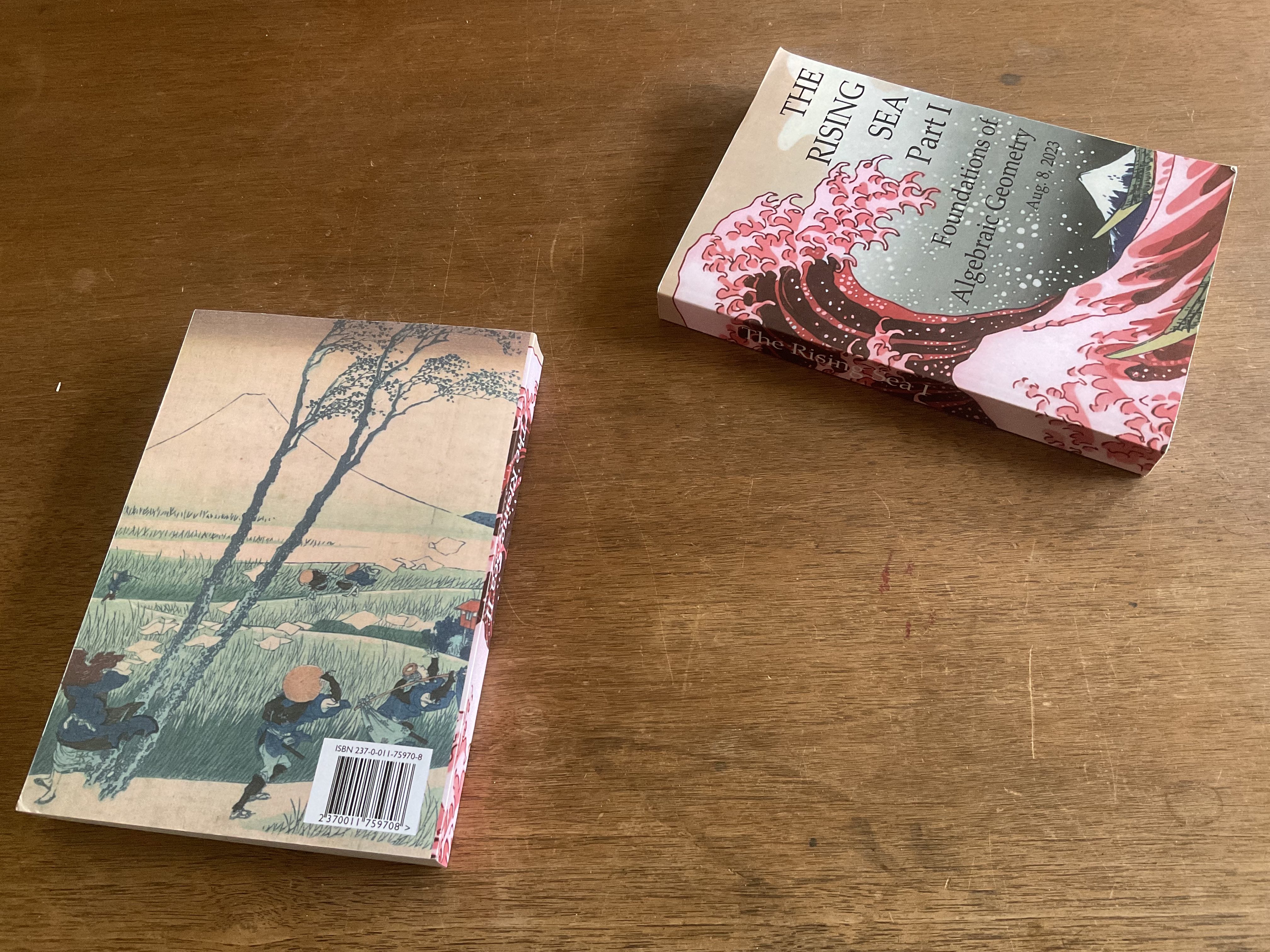
A new version of the notes is available at the usual place (the February 21 2024 version). Everything is in potentially nearly final form for an “official version”, except for typesetting/formatting and the index. 

---

(a) Significant change, but not substantive:  The figures are now basically done (meaning:  redone). Because I think people should be comfortable making their own sketches in real time as they figure things out, I’ve deliberately gone all in on a hand-drawn aesthetic. This is atypical, even amateurish, for serious mathematics books. So maybe I will reconsider.

(b) About composition of projective morphisms (the old Exercise 17.3.B), and more generally 17.3:  I realize now what the complication was in the old 17.3.B.  People were stuck at many steps, but the real issue was only the last one, to get to the quasicompact target case once you already had the target line bundle. There was indeed a gap there. Given what is done in the notes (and not even by this point in the version previously posted), we can show it only in the Noetherian case.  So the new version has 17.3 seriously rearranged in a number of ways.  In particular, now the old 17.3.B is a bit later, and the argument is for when the final target is either affine or Noetherian.  (Even this requires as a black box something that will only be proved in the cohomology chapter, which is Grothendieck’s coherence theorem for projective morphisms.)    I think this is now rigorous and complete. Please let me know if there are issues.  (Some of David Speyer’s ideas also in retrospect guided me on how to improve it.)  I’ve moved all the double-starred bits to the end (and I hope the reader ignores them all).  There is a single-starred section that is where the trouble lies, and that’s going to be hard going for those readers working through it.

(c) In the chapter on the 27 lines (you know which chapter number it is), I was always unhappy about needing Castelnuovo’s criterion.  János Kollár pointed an explicit workaround that I like a lot.  (I know that, roughly, doing it in this hands-on way, is very classical; but it is hard to do it rigorously without hand-waving, and you’ll notice this hand-waving in some expositions you may have seen.)  This is now Proof 2 of Proposition 27.4.1.  His explanation to me was direct and to the point; I’ve muddied it a little to fit the narrative, so the “worsening” is due to me.  (Most mathematicians have their own particular kind of thinking, which they are best at.  Kollár has this rather amazing ability of understanding very abstract things and very concrete things, both as well as anyone else, and those two things seem to be connected directly in his head in a way that they are not for most algebraic geometers. When I was in grad school, we secretly called him “The Mighty Kollár”, and even now it doesn’t seem an inappropriate name, although I would never say it to his face.) 

---

General philosophical point:  I’ve noticed that there is a tension between the kinds of requests people have of the notes.     Roughly, on one hand, there is my desire to try to make it possible to cover some central core of the material in a year (for at least some people), which requires rather severe compromises.  I’m trying to make different compromises than most people have made in the past (in particular, I’d like to expect less from the reader in terms of background, but then I need to expect more from the reader in other ways).  The things I need to push back against are things like “This topic really needs to be included”, “This topic needs to be fleshed out more completely”, “This topic is not done in sufficient generality”, “This topic needs to be done more rigorously”, “The presentation of this topic is well tuned to me as a reader”, “I coudn’t solve this exercise”.  In all of these cases, the suggestions are good ones, but at some point the manuscript will sink under the weight of items loaded onto it.  Usually those making suggestions are happy to suggest what other things should be cut, but you might not be surprised to hear that these suggestions contradict each other.    I’ve tried to help by starring and double-starring some topics, but I can’t seem to stop some readers from not skipping them (and then getting boggeddown).  I’ve had a number of suggestions of things that “really are needed in such a work” that I’ve had to repeatedly decline.  Even the ones I have said yes to have let it creep up to 850 pages even after the I passed a secret “no new material” line in my mind.  (Some recent additions:  on top of the ones mentioned above:  a brief mention of projective normality; definition of Cartier divisor in generality; and more.  But even these are things I think the reader can quickly read on their own from their web having read these notes, and needn’t be here.)

One form of the compromises I’ve made is:  “If we need it, I don’t want to black-box it, and I want you to understand it, but I only need you to understand it well enough to use it and move on”, and “if we don’t need it, no matter how wonderful it is, we should just skip it, and you can learn it on your own later” (so if included, those things are starred or double-starred).  I’ve had a hard time maintaining this position consistently, and over time a lot of things have slipped by my defenses.

At this point I am still entertaining all sorts of suggestions, but am going to try to stick to things that particularly deal with mathematical errors (often leaving imperfections and imprecisions — and many of these were actually deliberate choices), or really affect the understanding of a significant portion of readers (which I have some broader sense of given comments over the years) and not just you personally.

Many of the recent comments (including some still for me to think about) are here on this website.  Some excellent ones have come to me by email, from a group of students in Poland, by way of Joachim Jelisiejew.   I want mention them here, and I also look forward to seeing what these students go on to do mathematically in a few years’ time, because they are clearly very talented.

 

February 2024 version: content now complete, including index

A new version of the notes is available here. (It, and all older versions, are available at the usual place.) I don’t have much to report, but I just wanted to post the current version as it continues to converge. Please do continue sending in comments, particularly in the next month. There is a good chance that fairly soon a “snapshot” will be taken for an official publishable version (although that doesn’t mean that it will then be frozen).

In some more detail: I’ve now implemented the vast majority of the ideas from suggestions people have given, although there are some still to go. I’m redoing the figures in a consistent style, and about 2/3 of them are redone so far. The index will get some attention later, but the raw material is there, and I welcome suggestions and corrections. The only things I’m not interested in are latex issues (margins, etc.; but typos and errors in spacing are fair game). I am now ready for comments on figures, although there are still 1/3 of them that I haven’t re-done. 

I’ll very be busy with other duties for the next four years, so I will be able to spend much less time and attention on this. I suspect it will be enough of a break that I won’t be able to return afterwards with everything as fully in my head as it is now, so this will likely be my last chance for me to really make this as good as it can be before letting it go off into the world on its own. This really feels like nearing the endgame.

So thank you all for accompanying me on this stage of what has been a most interesting and rewarding journey for me.

 

July 2023 version: content now complete, including index

A new version of the notes is available here. (It, and all older versions, are available at the usual place.) The main change from the previous version: The index is potentially done.

Now the editing I will do will be primarily in response to comments and suggestions from others. I am very interested in any suggestions and corrections you may have (including things you told me before that I have forgotten). The only things I’m not interested in are: latex issues (margins, etc.; but typos and errors in spacing are fair game) and ugliness of figures (but content of figures is fair game).

 

June 2023 version: potentially finalized content

A new version of the notes is available here. (It, and all older versions, are available at the usual place.) For the first time, I would say that the content and editing is “potentially done”. All content is potentially polished. (Not done: beautification issues e.g. fighting with latex over line breaks. And the index is very rough.) I am thus very interested in any suggestions and corrections you may have, including things you told me before. (I think I’ve implemented all the edits from my to-do list from comments you have made through the years, by email or here on this site.)

In more detail: This is a fairly substantial revision. I also taught from the notes in the last two quarters, and the excellent comments of the excellent people in the class helped tremendously.    I may not do much more before I declare this project “done”.

New arguments added recently (perhaps in the last few revisions):

• a scheme with no closed points, and a little more about coproducts
• fixed proof of Serre duality (long in coming)
• a glimpse of the Koszul complex, and proof of the Hilbert Syzygy Theorem (I learned how to think about this from Michael Kemeny)
• improved exposition of proof of formal function theorem (unlike other cases, really the same proof)
• all the important flatness facts are now done much more easily
• and many more things I can’t remember right now.

I’m definitely looking for any small remaining issues.  And also any mathematical mistakes or omissions.   

A random cool thing I wanted to share: I have always wanted a way to order mathematical notes, in perhaps a semi-public way or a private way, that would be nonlinear and easy and robust. Wikis are good but have some imperfections. The “back end” of the stacks project (gerby) is fantastic for public presentation of huge amounts of interconnected material, but less suited to person note-taking because it is somewhat fragile, and has significant start-up time to use properly. (For more on gerby, see: https://gerby-project.github.io/ .) I stumbled on Jon Sterling’s “forest”, and I can do nothing better than just point you here: https://forest.jonmsterling.com/index.xml and recommend that you take a look and explore. He has done a lot of thinking on “tools for mathematical thought”, which is precisely the the sort of thing I was wanting to think through more myself. It is something akin to a manifesto. (As is unfortunately common as many of you know, I owe him an email.) I would like to explore this further (despite extreme lack of time), and I wanted to advertise this, in case others would like to try it out too!

 

April 2023 version of the notes

A new version of the notes is available here. (It, and all older versions, are available at the usual place.)

Supravat Sarkar kindly pointed out that my Chevalley’s Theorem proof was still flawed at the very last step. I have now, I think (again!) fixed it. See Section 8.4.4 for that.

 

(i) reference question (pathological non-Noetherian examples), and (ii) the Jordan-Holder package

Update to the notes: I will probably post a new version of The Rising Sea notes after our quarter ends. By the end of two quarters of the three-quarter sequence this year, we will reach the end of the chapter on curves, and there are only around ten known issues in the notes I want to fix up until that point. (But there are a triple-digit number of issues afterwards, which I hope to make serious progress on next quarter!)

(i) I’d like to give explicit references to examples of what behavior can go seriously wrong in the non-Noetherian setting, and long ago I’d scribbled some notes, but now I can’t remember what the actual references were to. Can anyone point me to where these are in the literature (because I’m sure I’ve seen them)? I had thought they were in the stacks project, but couldn’t easily find them there. The right person to ask is the incomparable Johan de Jong, and I can email him later, but I thought I may as well ask here first.

(a) There is a projective flat morphism where the fiber dimension is not locally constant.

(b) There is a finite flat morphism where the degree of the fiber is not locally constant.

(c) There is a projective flat morphism where the fibers are curves, and the arithmetic genus is not locally constant.

(d) There is a projective morphism for which the pushforward of coherent sheaves are not always coherent.

Behind these might be the famous “five-pound” counter-examples in the stacks project (aka tag 05LB, and now you can never forget its tag), based on a ring R with an ideal I such that R/I is flat but not projective. It is easy to describe R and I: R are the infinitely differentiable functions on the real numbers, and I are those functions that vanish in an open neighborhood of zero.

These examples are really unimportant in general in some sense, but I like having a strong sense of where the boundaries of civilization are, and what kinds of monsters actually live beyond those boundaries.

(ii) In return, I’ll give a sample new brief section. I realize now that I’ve been teaching and understanding the Jordan-Holder theorem wrong in group theory (way back in “introduction to group theory”). I’m now going to teach it in a way that naturally leads you to the notion of length, and simple objects in more general categories (without using those words), in a more natural way. One day I would like to write it up as a “bedtime story” in the style of what I did for exact sequences here. But I here is the write-up in a short section in the current version of The Rising Sea. I want it to be friendly and easy (for someone reading The Rising Sea, not someone seeing group theory the first time).

jordanholdermar1123Download

Incidentally, we traditionally teach/present the groups/rings/fields/modules class/material in the order “groups, then rings, then perhaps some modules or fields, then move from there”. I think I will next try to do it: “you know linear algebra, so let’s define a field, and vector space together, then start the course with abelian groups and their actions (leading to quotients etc., ie experience with the abelian category package extending vector spaces), then rings, then a touch of modules (and quotients etc), then UFDs, PIDs, Smith normal form from which we get classification of finitely generated abelian groups. Only then, to general groups, actions, quotients (with added weirdness). I would have to not give up any “canonical” material in the class (Math 120 at Stanford) in order to set them up for the next class, but I think I could do it. Unsurprisingly, I like Paolo Aluffi‘s approach (his homepage has a picture of the tree in which he lives); he told me last week he also does largely follows this path, although he actually does rings first. (It seems logically harder than doing abelian groups first, but conceptually I think he is right that it is easier, because people will already have an excellent intuition for the integers to build on.) He does this in his book Algebra: Notes from the Underground, which is in keeping with the excellent philosophy of his book Algebra: Chapter 0.

 

December 2022 version of the notes

Happy New Year! The picture is of an amazing artwork by Gabriel Dorfsman-Hopkins and Daniel Rostamloo of 27 lines on a cubic surface. Here is a link to the webpage for the sculpture.

The latest (December 31, 2022 version) of the notes are posted here, at the usual place. In terms of content, it remains (and will remain) very similar to the previous version. But it has been substantially edited and polished.

In more detail: the first 18 chapters are much more polished than before, and are nearly in “potentially final form”. Most of the later chapters are still waiting for that level of tender loving care. Please continue to let me know a$bout any suggestions, corrections, typos, etc., in any chapter, no matter how small. The only exceptions are stylistic things (margins, fonts, low-quality figures).

Here are some changes I find interesting or worth mentioning.

Chapter 8: The Chevalley’s Theorem proof still had a small flaw, and is now fixed. (Thanks to Hikari Iwasaki for comments on this and many other things near there.) It is now one that I find so natural that I can’t forget it, and can easily explain while walking across the quad.

Chapter 10: The starred section, and doubled-starred proofs, on things like “geometrically reduced/integral/etc.” have been awaiting patching for a very long time. I finally did it. If you are curious, or want to solidify your understanding of those issues, please take a look. I hope that it has become very comprehensible. The main black box (that I punted to the chapter on flatness) is that if is any -scheme, then is universally open.

Chapter 12: The chapter on dimension is substantially rewritten, and I hope it is a cleaner way through the topic. There are some explanations directly or indirectly from Mel Hochster and Qing Liu. (I highly recommend Qing Liu’s book; I love how he thinks in a very “clean” way.)

Chapter 13: I had been meaning to rethink the older version of the chapter on regularity and smoothness for some time. I’ve now done so, and fixed a lot of problems. I know from experience that I have undoubtedly introduced new ones. From the new point of view, the central players here is that if you want to get at notions of regularity and smoothness, you are led to the notion of the Zariski tangent space and the Jacobian criterion, and everything revolves around them.

Chapter 15: If there is a single central fulcrum on which everything balances, it is at the almost literal center of the notes: the link between line bundles and divisors. This is a tricky topic the first time you see it, and section 15.2 has always been trickier for readers than I want it to be. I hope it is better now.

Also, Pol van Hoften told me the definition of abelian category which he prefers, and I was very surprised to find it much clearer and enlightening than anything I had known before. How could this be, given how old and important a notion it is? Pol’s definition is from Jacob Lurie’s Higher Algebra, although his description of it is his own. I have now included it in the notes. I’ll tell you it here, because it is something directly memorable enough that (unlike the previous definition) I can remember it without trying. Also, I learned something new: the notion of abelian category is intrinsic to the category itself — there is no additional structure required. That was so unclear from other definitions that I did not realize it despite using this notion for years! Here is Pol’s description. We are motivated by the abelian categories we already know and love. Suppose is a category. We give some axioms that determine whether it is an additive category, or an abelian category.

Axiom 0: has a zero object (an object that is both final and initial). Of course this axiom should be numbered zero. And of course abelian categories need a zero object, so this is easy to remember.

For the next axioms, we note that abelian categories have finite products and coproducts, and they are the same. Let’s axiomatize this.

Axiom 1: For any two objects and , the product and coproduct exists. (Hence has finite products and coproducts.)

Axiom 2: By the universal property of product and coproduct, we therefore have a map for all pairs of objects. We require that this map be an isomorphism.

Now here is the insight I didn’t realize: with this information, we can discover how to “add” two morphisms from to . And adding the zero morphism (the morphism that factors through the 0 object) does nothing under this operation. You can check that this gives intrinsically the structure of a commutative monoid (it is associative, has identity). And it even automatically distributes in the way we’d like (e.g., if we have two maps and from to , and one map , then ). It is fun seeing how some of these work out.

We don’t yet know that it is an abelian group, because we don’t know that + has an inverse. So that is our next axiom.

Axiom 3. For any two objects and , this operation + gives the structure of an abelian group.

At this point we have defined the notion of additive category. Note that we don’t require that have the structure of an abelian group (which I used to think of as an additional structure); we have the property that with its pre-existing operation + is such that + has an inverse.

Axiom 4 and 5 are just the two axioms making additive categories into abelian categories. Axiom 4: kernels and cokernels exist. Axiom 5: some property (you can have several choices here, leading to the same definition) that kernels and cokernels have to satisfy. Usually it is “some property and its dual”. Once again, there is no additional structure required; just a condition.

So if you have two abelian categories and , and you have a functor , how do you know if it is a map of abelian categories? All you need to do is to check that it preserves products and coproducts (of two elements) and kernels and cokernels. All other parts of the structure come at no extra charge.

I will teach the second and third quarters of “Foundations of Algebraic Geometry” this winter and spring quarters (Pol taught the first one and by all accounts did a remarkable job). I hope to continue to edit the file during this time, and clean up more chapters.

 

August 2022 version of the notes

It has been a while, but finally, the next version of the notes are here. (For convenience, all earlier versions are posted at the usual place. Added Sept. 4, 2022: a version with an imperfect index is here.)

It took a while because I split the quasicoherent sheaves chapter in two (one is much earlier, and is quasicoherent sheaves ~ “modules over a ring”, and the later one is quasicoherent sheaves ~ “vector bundles”), which required a cascading series of changes in logic and ordering and references.

But it is in much better shape, and I intend to post updates periodically this academic year. People have given me a large number of very useful comments, and they are all in the process of being considered (and often implemented). I think comments made on this blog have been mostly responded (even if to say “it is now on the list”).

Please continue to let me know about any suggestions, corrections, typos, etc., no matter how small. The only exceptions are stylistic things (margins, fonts, low-quality figures).

At this point the figures are supposed to now be substantively correct (except of course where there are things on my “to do list” to fix). Everything before the chapter on dimension now has essentially no remaining known issues (except for a few pages on geometric fibers that I am still rewriting). Later chapters are in different stages of editing.

Here are some random notable changes that I can remember off the top of my head — the things mentioned in earlier posts (associated points; cohomology and base change; etc.) are now in. I like the proof of Chevalley’s Theorem much better (it feels now very easy modulo the fact that finite morphisms are closed).

 

A fun example from Daniel Litt: slightly unusual behavior of infinite rank vector bundles

Suppose is a short exact sequence of quasicoherent sheaves.     If two out of three of are locally free, what can we say about the third?  

If and are locally free, then need not be.    This is a fundamental example.

If and are locally free, then is too.    This is important and not too hard.

If and are locally free and finite rank, then is too.  This is also useful.

But if and are locally free, and infinite rank, then need not be locally free.  The purpose of this post is to give Daniel Litt‘s explanation to me of a simple example of this.  I thought this example was not right to include in the Rising Sea (it would be distracting), but I wanted to preserve it for posterity (and for myself).

I will describe a surjective map of free modules whose kernel is not locally free. Viewed geometrically, this provides a surjective map of trivial (infinite-dimensional) vector bundles whose kernel is not a vector bundle. Of course, the kernel is projective.

Let be a projective module over a ring which is not locally free.  (Such things exist, see for example the Stacks Project tag 05WG.  To be explicit, there and is the ideal (where there are 1’s).)

Then is a direct summand of a free module, say .  Writing

gives as a direct summand of a free module with free complement. Then there is a short exact sequence

exhibiting as the kernel of a surjective map of free modules, where the map is the projection.

 

Cohomology and base change: new exposition

A couple of posts ago, I gave the slick proof of cohomology and base change that I learned from Eric Larson (and that to the best of my knowledge should be credited to him). Here is the rewritten chapter on cohomology and base change, now only 17 pages long, which incorporates his argument (as well as various other corrections and suggestions people have sent through the years).

ch28jul1522Download

As always, I’m happy to hear of any errors/typos/suggestions!